Chapter 2 Bias in the Data (Risk of Recidivism Analysis)
2.1 Setup
## Loading required package: pacmanpacman::p_load(
tidyverse, # tidyverse packages
conflicted, # an alternative conflict resolution strategy
ggthemes, # other themes for ggplot2
patchwork, # arranging ggplots
scales, # rescaling
survival, # survival analysis
broom, # for modeling
here, # reproducibility
glue # pasting strings and objects
)
# To avoid conflicts
conflict_prefer("filter", "dplyr") ## [conflicted] Will prefer dplyr::filter over any other package## [conflicted] Will prefer dplyr::select over any other package2.2 Load data
We select fields for severity of charge, number of priors, demographics, age, sex, COMPAS scores, and whether each person was accused of a crime within two years.
## Warning: Duplicated column names deduplicated: 'decile_score' =>
## 'decile_score_1' [40], 'priors_count' => 'priors_count_1' [49]## N of observations (rows): 7214
## N of variables (columns): 532.3 Wrangling
- Not all of the observations are useable for the first round of analysis.
- There are a number of reasons to remove rows because of missing data:
- If the charge date of a defendants COMPAS scored crime was not within 30 days from when the person was arrested, we assume that because of data quality reasons, that we do not have the right offense.
- We coded the recidivist flag – is_recid – to be -1 if we could not find a COMPAS case at all.
- In a similar vein, ordinary traffic offenses – those with a c_charge_degree of ‘O’ – will not result in Jail time are removed (only two of them).
- We filtered the underlying data from Broward county to include only those rows representing people who had either recidivated in two years, or had at least two years outside of a correctional facility.
2.3.1 Create a function
wrangle_data <- function(data){

df <- data %>%

    # Select variables
    select(age, c_charge_degree, race, age_cat, score_text, sex, priors_count, days_b_screening_arrest, decile_score, is_recid, two_year_recid,
         c_jail_in, c_jail_out) %>%
    # Filter rows
    filter(days_b_screening_arrest <= 30,
           days_b_screening_arrest >= -30,
           is_recid != -1,
           c_charge_degree != "O",
           score_text != 'N/A') %>%
    # Mutate variables
    mutate(length_of_stay = as.numeric(as.Date(c_jail_out) - as.Date(c_jail_in)),
           c_charge_degree = factor(c_charge_degree),
           age_cat = factor(age_cat),
           race = factor(race, levels = c("Caucasian","African-American","Hispanic","Other","Asian","Native American")),
           sex = factor(sex, levels = c("Male","Female")),
           score_text = factor(score_text, levels = c("Low", "Medium", "High")),
           score = score_text,
# I added this new variable to test whether measuring the DV as a binary or continuous var makes a difference
           score_num = as.numeric(score_text)) %>%
    # Rename variables
    rename(crime = c_charge_degree,
           gender = sex)

return(df)}
2.3.2 Apply the function to the data
##  [1] "age"                     "crime"
##  [3] "race"                    "age_cat"
##  [5] "score_text"              "gender"
##  [7] "priors_count"            "days_b_screening_arrest"
##  [9] "decile_score"            "is_recid"
## [11] "two_year_recid"          "c_jail_in"
## [13] "c_jail_out"              "length_of_stay"
## [15] "score" "score_num"## # A tibble: 5 x 16
## age crime race age_cat score_text gender priors_count days_b_screenin…
## <dbl> <fct> <fct> <fct> <fct> <fct> <dbl> <dbl>
## 1 69 F Other Greate… Low Male 0 -1
## 2 34 F Afri… 25 - 45 Low Male 0 -1
## 3 24 F Afri… Less t… Low Male 4 -1
## 4 44 M Other 25 - 45 Low Male 0 0
## 5 41 F Cauc… 25 - 45 Medium Male 14 -1
## # … with 8 more variables: decile_score <dbl>, is_recid <dbl>,
## # two_year_recid <dbl>, c_jail_in <dttm>, c_jail_out <dttm>,
## # length_of_stay <dbl>, score <fct>, score_num <dbl>2.4 Descriptive analysis
- Higher COMPAS scores are slightly correlated with a longer length of stay.
## [1] 0.2073297df %>%
group_by(score) %>%
count() %>%
ggplot(aes(x = score, y = n)) +
geom_col() +
labs(x = "Score",
y = "Count",
title = "Score distribution")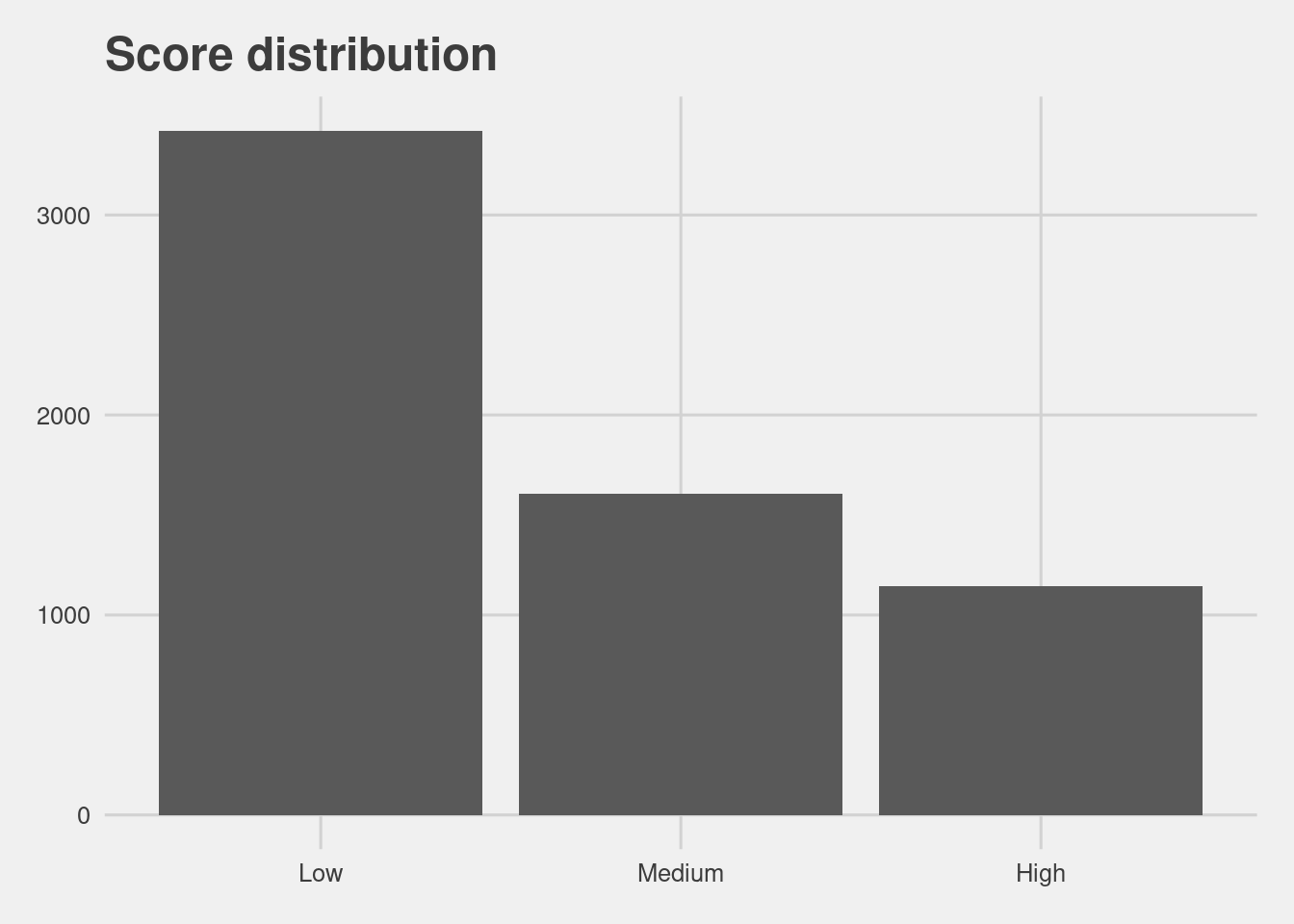 Judges are often presented with two sets of scores from the COMPAS system – one that classifies people into High, Medium and Low risk, and a corresponding decile score. There is a clear downward trend in the decile scores as those scores increase for white defendants.
df %>%
  ggplot(aes(ordered(decile_score))) +
          geom_bar() +
          facet_wrap(~race, nrow = 2) +
          labs(x = "Decile Score",
               y = "Count",
               Title = "Defendant's Decile Score")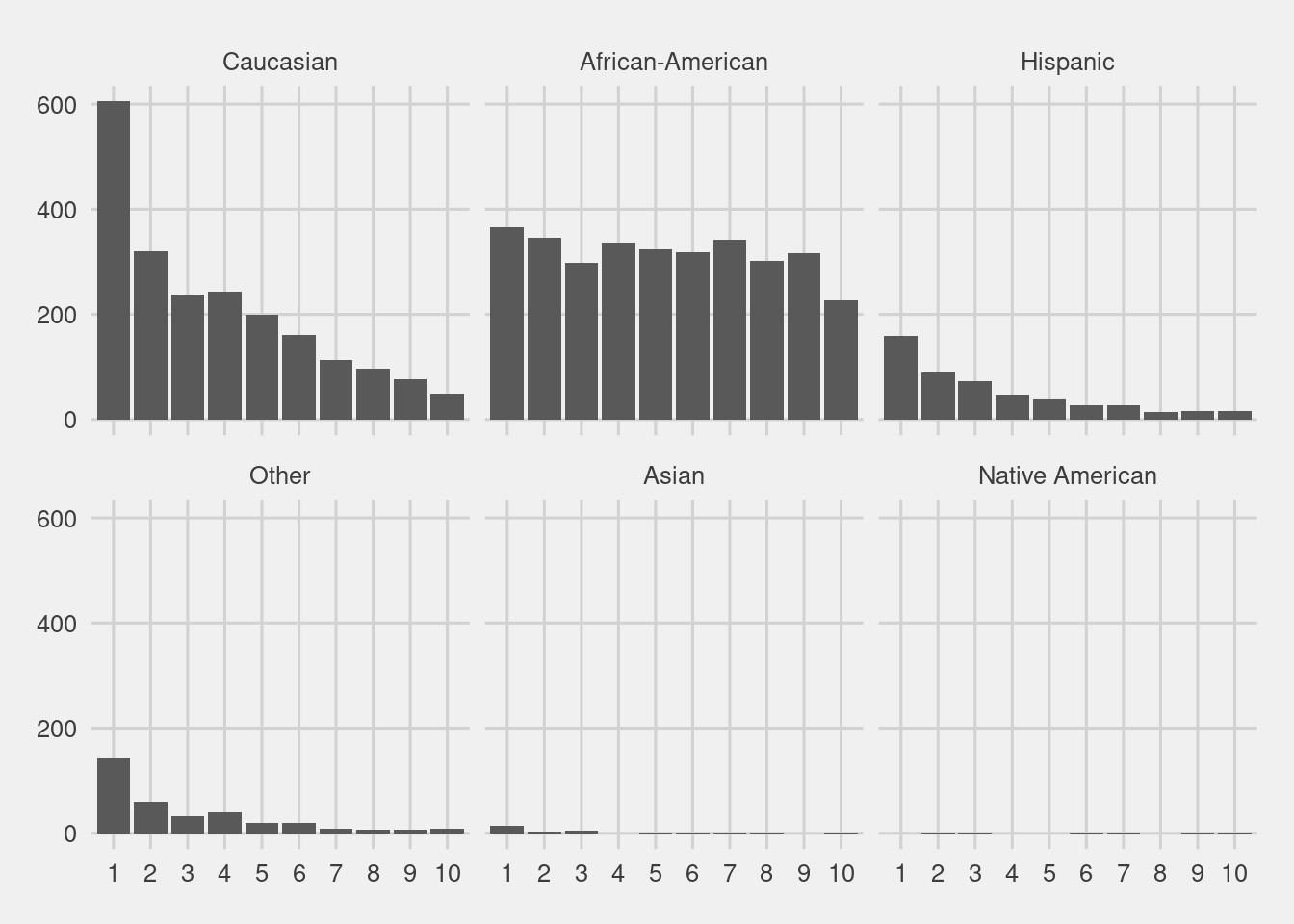
2.5 Modeling
After filtering out bad rows, our first question is whether there is a significant difference in COMPAS scores between races. To do so we need to change some variables into factors, and run a logistic regression, comparing low scores to high scores.
2.5.1 Model building
model_data <- function(data){

# Logistic regression model
lr_model <- glm(score ~ gender + age_cat + race + priors_count + crime + two_year_recid,
             family = "binomial", data = data)

# OLS, DV = score_num
ols_model1 <- lm(score_num ~ gender + age_cat + race + priors_count + crime + two_year_recid, data = data)

# OLS, DV = decile_score
ols_model2 <- lm(decile_score ~ gender + age_cat + race + priors_count + crime + two_year_recid, data = data)

# Extract model outcomes with confidence intervals
lr_est <- lr_model %>%
    tidy(conf.int = TRUE)

ols_est1 <- ols_model1 %>%
    tidy(conf.int = TRUE)

ols_est2 <- ols_model2 %>%
    tidy(conf.int = TRUE)

# AIC scores
lr_AIC <- AIC(lr_model)
ols_AIC1 <- AIC(ols_model1)
ols_AIC2 <- AIC(ols_model2)

list(lr_est, ols_est1, ols_est2,
     lr_AIC, ols_AIC1, ols_AIC2)

}
2.5.2 Model comparisons
glue("AIC score of logistic regression: {model_data(df)[4]}
      AIC score of OLS regression (with categorical DV):  {model_data(df)[5]}
      AIC score of OLS regression (with continuous DV): {model_data(df)[6]}")
## AIC score of logistic regression: 6192.40169473357
## AIC score of OLS regression (with categorical DV): 11772.1148541111
## AIC score of OLS regression (with continuous DV): 26779.95122269992.5.3 Logistic regression model
lr_model <- model_data(df)[1] %>% data.frame()

lr_model %>%
  filter(term != "(Intercept)") %>%
  mutate(term = gsub("race|age_cat|gender|M","", term)) %>%
  ggplot(aes(x = fct_reorder(term, estimate), y = estimate, ymax = conf.high, ymin = conf.low)) +
  geom_pointrange() +
  coord_flip() +
  labs(y = "Estimate", x = "",
      title = "Logistic regression") +
  geom_hline(yintercept = 0, linetype = "dashed")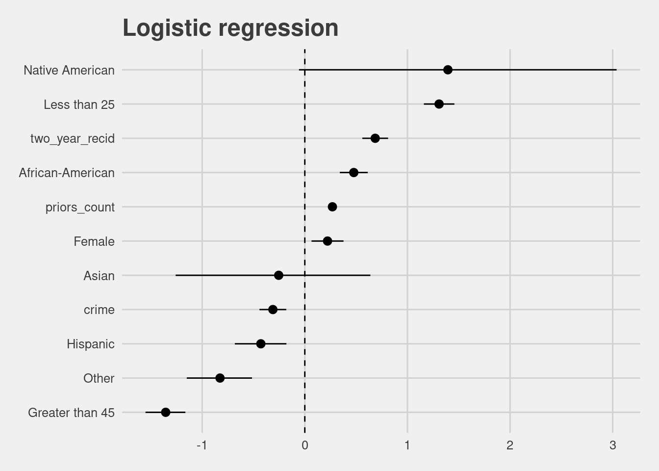
Logistic regression coefficients are log odds ratios. Remember an odd is \(\frac{p}{1-p}\). p could be defined as a success and 1-p could be as a failure. Here, coefficient 1 indicates equal probability for the binary outcomes. Coefficient greater than 1 indicates strong chance for p and weak chance for 1-p. Coefficient smaller than 1 indicates the opposite. Nonetheless, the exact interpretation is not very interpretive as an odd of 2.0 corresponds to the probability of 1/3 (!).
(To refresh your memory, note that probability is bounded between [0, 1]. Odds ranges between 0 and infinity. Log odds ranges from negative to positive infinity. We’re going through this hassle because we used log function to map predictor variables to probability to fit the model to the binary outcomes.)
In this case, we reinterpret coefficients by turning log odds ratios into relative risks. Relative risk = odds ratio / 1 - p0 + (p0 * odds ratio) p-0 is the baseline risk. For more information on relative risks and its value in statistical communication, see Grant (2014), Wang (2013), and Zhang and Yu (1998).
odds_to_risk <- function(model){

    # Calculating p0 (baseline or control group)
    intercept <- model$estimate[model$term == "(Intercept)"]
    control <- exp(intercept) / (1 + exp(intercept))

    # Calculating relative risk
    model <- model %>% filter(term != "(Intercept)")
    model$relative_risk <- (exp(model$estimate) /
                        (1 - control + (control * exp(model$estimate))))

    return(model)
}## relative_risk term estimate std.error statistic
## 1 2.6152880 raceNative American 1.3942077 0.76611816 1.8198338
## 2 2.4961195 age_catLess than 25 1.3083903 0.07592869 17.2318308
## 3 1.6882587 two_year_recid 0.6858625 0.06401955 10.7133288
## 4 1.4528374 raceAfrican-American 0.4772070 0.06934914 6.8812245
## 5 1.2402135 priors_count 0.2689453 0.01110379 24.2210342
## 6 1.1947947 genderFemale 0.2212667 0.07951020 2.7828714
## 7 0.8077863 raceAsian -0.2544147 0.47821105 -0.5320135
## 8 0.7692955 crimeM -0.3112408 0.06654750 -4.6769729
## 9 0.6948050 raceHispanic -0.4283949 0.12812549 -3.3435572
## 10 0.4865228 raceOther -0.8263469 0.16208006 -5.0983873
## 11 0.2971899 age_catGreater than 45 -1.3556332 0.09908053 -13.6821355
## p.value conf.low conf.high
## 1 6.878432e-02 -0.05694017 3.0383160
## 2 1.532239e-66 1.16008750 1.4577645
## 3 8.813460e-27 0.56039880 0.8113799
## 4 5.934025e-12 0.34137020 0.6132514
## 5 1.335783e-129 0.24750487 0.2910343
## 6 5.388016e-03 0.06532360 0.3770591
## 7 5.947167e-01 -1.25877950 0.6389894
## 8 2.911407e-06 -0.44178937 -0.1808904
## 9 8.271164e-04 -0.68190124 -0.1794075
## 10 3.425594e-07 -1.15026143 -0.5142075
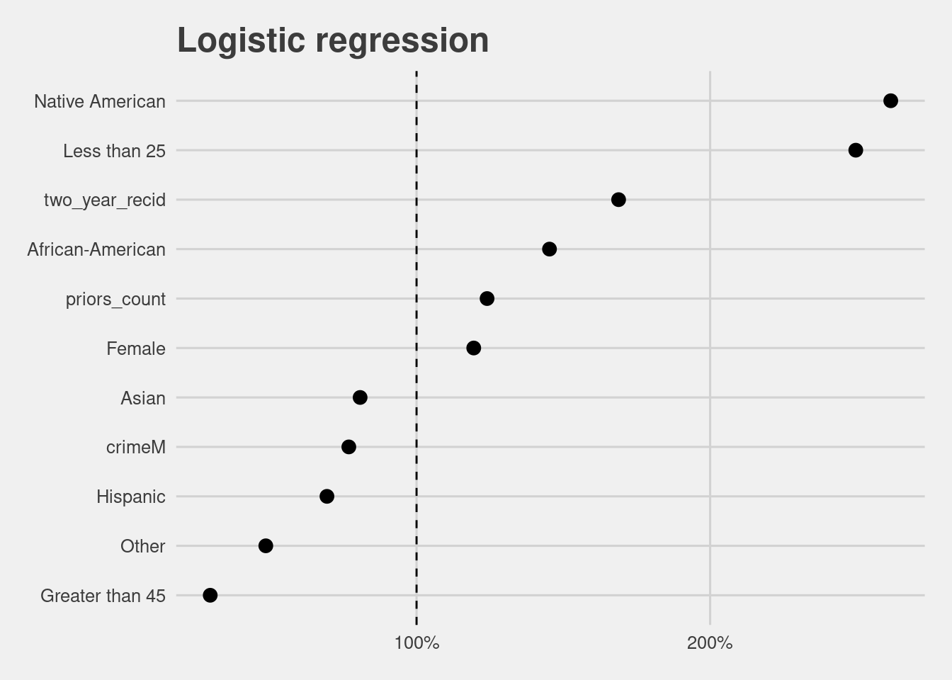
## 11 1.298233e-42 -1.55226716 -1.1637224Relative risk score 1.45 (African American) indicates that black defendants are 45% more likely than white defendants to receive a higher score.
The plot visualizes this and other results from the table.
odds_to_risk(lr_model) %>%
    mutate(term = gsub("race|age_cat|gender","", term)) %>%
    ggplot(aes(x = fct_reorder(term, relative_risk), y = relative_risk)) +
        geom_point(size = 3) +
        coord_flip() +
        labs(y = "Likelihood", x = "",
             title = "Logistic regression") +
        scale_y_continuous(labels = scales::percent_format(accuracy = 1)) +
        geom_hline(yintercept = 1, linetype = "dashed")