Chapter 3 Bias in the Data (Risk of Violent Recidivism Analysis)
3.1 Setup
## Loading required package: pacmanpacman::p_load(
tidyverse, # tidyverse packages
conflicted, # an alternative conflict resolution strategy
ggthemes, # other themes for ggplot2
patchwork, # arranging ggplots
scales, # rescaling
survival, # survival analysis
broom, # for modeling
here, # reproducibility
glue # pasting strings and objects
)
# To avoid conflicts
conflict_prefer("filter", "dplyr") ## [conflicted] Will prefer dplyr::filter over any other package## [conflicted] Will prefer dplyr::select over any other package3.2 Load data
## Warning: Duplicated column names deduplicated: 'decile_score' =>
## 'decile_score_1' [40], 'priors_count' => 'priors_count_1' [49], 'two_year_recid'
## => 'two_year_recid_1' [54]
##
## ── Column specification ────────────────────────────────────────────────────────────────────────────
## cols(
## .default = col_double(),
## name = col_character(),
## first = col_character(),
## last = col_character(),
## compas_screening_date = col_date(format = ""),
## sex = col_character(),
## dob = col_date(format = ""),
## age_cat = col_character(),
## race = col_character(),
## c_jail_in = col_datetime(format = ""),
## c_jail_out = col_datetime(format = ""),
## c_case_number = col_character(),
## c_offense_date = col_date(format = ""),
## c_arrest_date = col_date(format = ""),
## c_charge_degree = col_character(),
## c_charge_desc = col_character(),
## r_case_number = col_character(),
## r_charge_degree = col_character(),
## r_offense_date = col_date(format = ""),
## r_charge_desc = col_character(),
## r_jail_in = col_date(format = "")
## # ... with 14 more columns
## )
## ℹ Use `spec()` for the full column specifications.glue("N of observations (rows): {nrow(two_years_violent)}
N of variables (columns): {ncol(two_years_violent)}")## N of observations (rows): 4743
## N of variables (columns): 543.3 Wrangling
3.3.1 Create a function
wrangle_data <- function(data){

df <- data %>%

    # Select variables
    select(age, c_charge_degree, race, age_cat, v_score_text, sex, priors_count,
         days_b_screening_arrest, v_decile_score, is_recid, two_year_recid) %>%
    # Filter rows
    filter(days_b_screening_arrest <= 30,
           days_b_screening_arrest >= -30,
           is_recid != -1,
           c_charge_degree != "O",
           v_score_text != 'N/A') %>%
    # Mutate variables
    mutate(c_charge_degree = factor(c_charge_degree),
           age_cat = factor(age_cat),
           race = factor(race, levels = c("Caucasian","African-American","Hispanic","Other","Asian","Native American")),
           sex = factor(sex, levels = c("Male","Female")),
           v_score_text = factor(v_score_text, levels = c("Low", "Medium", "High")),
# I added this new variable to test whether measuring the DV as a binary or continuous var makes a difference
           score_num = as.numeric(v_score_text)) %>%
    # Rename variables
    rename(crime = c_charge_degree,
           gender = sex,
           score = v_score_text)

return(df)}
3.3.2 Apply the function to the data
##  [1] "age"                     "crime"
##  [3] "race"                    "age_cat"
##  [5] "score"                   "gender"
##  [7] "priors_count"            "days_b_screening_arrest"
##  [9] "v_decile_score"          "is_recid"
## [11] "two_year_recid" "score_num"## # A tibble: 5 x 12
## age crime race age_cat score gender priors_count days_b_screenin…
## <dbl> <fct> <fct> <fct> <fct> <fct> <dbl> <dbl>
## 1 69 F Other Greate… Low Male 0 -1
## 2 34 F Afri… 25 - 45 Low Male 0 -1
## 3 44 M Other 25 - 45 Low Male 0 0
## 4 43 F Other 25 - 45 Low Male 3 -1
## 5 39 M Cauc… 25 - 45 Low Female 0 -1
## # … with 4 more variables: v_decile_score <dbl>, is_recid <dbl>,
## # two_year_recid <dbl>, score_num <dbl>3.3.3 Descriptive analysis
Score distribution
df %>%
  group_by(score) %>%
  count() %>%
  ggplot(aes(x = score, y = n)) +
    geom_col() +
    labs(x = "Score",
         y = "Count",
         title = "Score distribution")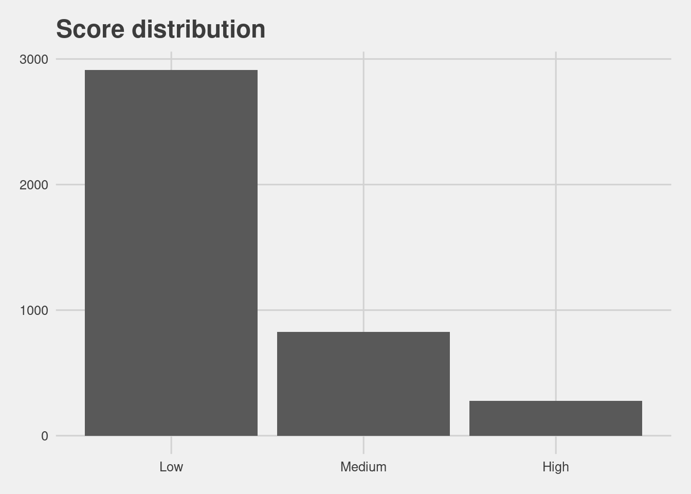
Score distribution by race
df %>%
  ggplot(aes(ordered(v_decile_score))) +
          geom_bar() +
          facet_wrap(~race, nrow = 2) +
          labs(x = "Decile Score",
               y = "Count",
               Title = "Defendant's Decile Score")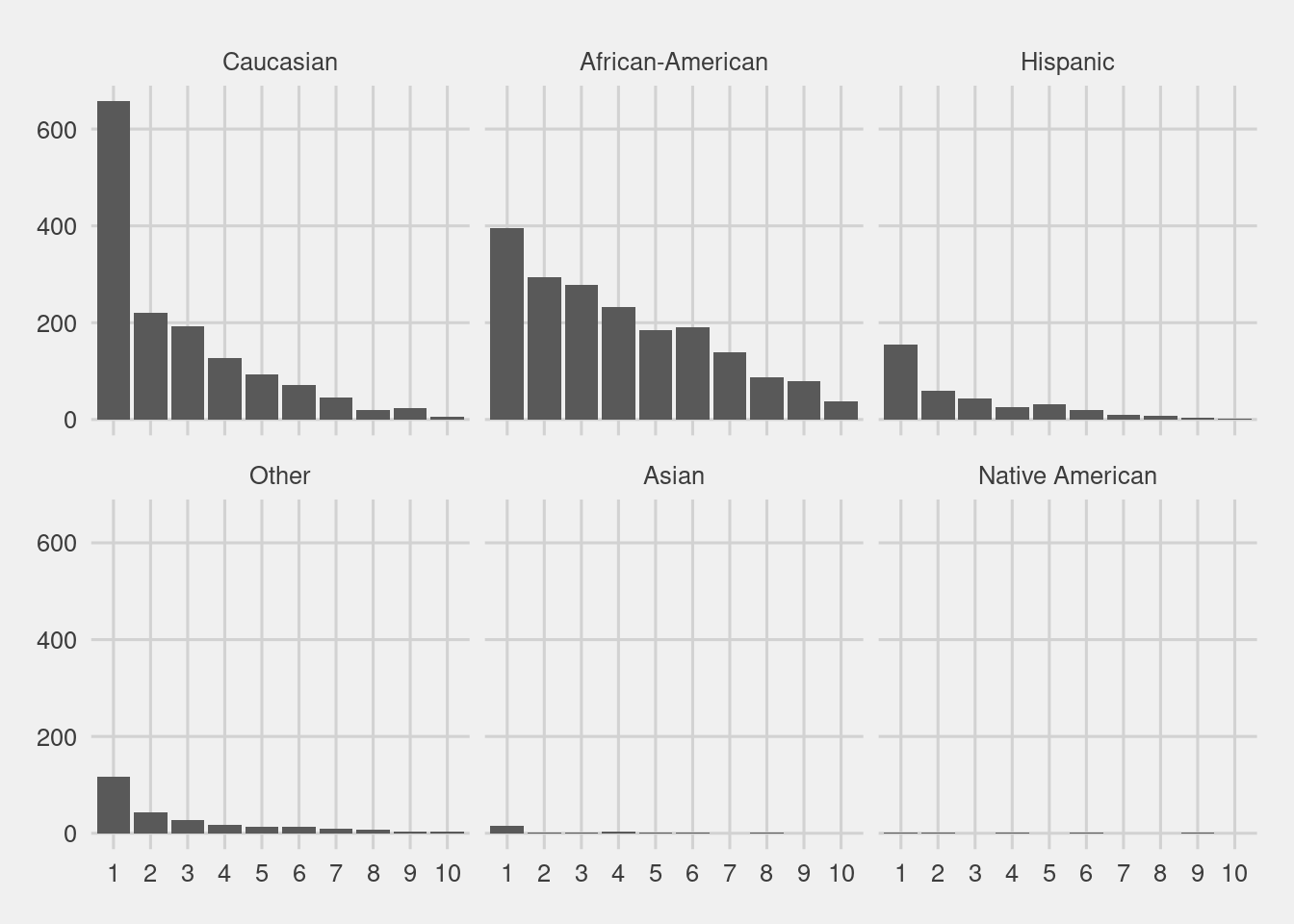
3.4 Modeling
After filtering out bad rows, our first question is whether there is a significant difference in COMPAS scores between races. To do so we need to change some variables into factors, and run a logistic regression, comparing low scores to high scores.
model_data <- function(data){

# Logistic regression model
lr_model <- glm(score ~ gender + age_cat + race + priors_count + crime + two_year_recid,
             family = "binomial", data = data)

# OLS
ols_model1 <- lm(score_num ~ gender + age_cat + race + priors_count + crime + two_year_recid,
             data = data)

ols_model2 <- lm(v_decile_score ~ gender + age_cat + race + priors_count + crime + two_year_recid,
             data = data)

# Extract model outcomes with confidence intervals
lr_est <- lr_model %>%
    tidy(conf.int = TRUE)

ols_est1 <- ols_model1 %>%
    tidy(conf.int = TRUE)

ols_est2 <- ols_model2 %>%
    tidy(conf.int = TRUE)

# AIC scores
lr_AIC <- AIC(lr_model)
ols_AIC1 <- AIC(ols_model1)
ols_AIC2 <- AIC(ols_model2)

list(lr_est, ols_est1, ols_est2, lr_AIC, ols_AIC1, ols_AIC2)
}
3.4.1 Model comparisons
glue("AIC score of logistic regression: {model_data(df)[4]}
      AIC score of OLS regression (with categorical DV):  {model_data(df)[5]}
      AIC score of OLS regression (with continuous DV): {model_data(df)[6]}")
## AIC score of logistic regression: 3022.77943765996
## AIC score of OLS regression (with categorical DV): 5414.49127581608
## AIC score of OLS regression (with continuous DV): 15458.38617231063.4.2 Logistic regression model
lr_model <- model_data(df)[1] %>%
  data.frame()

lr_model %>%
  filter(term != "(Intercept)") %>%
  mutate(term = gsub("race|age_cat|gender","", term)) %>%
  ggplot(aes(x = fct_reorder(term, estimate), y = estimate, ymax = conf.high, ymin = conf.low)) +
  geom_pointrange() +
  coord_flip() +
  labs(y = "Estimate", x = "",
      title = "Logistic regression") +
  geom_hline(yintercept = 0, linetype = "dashed")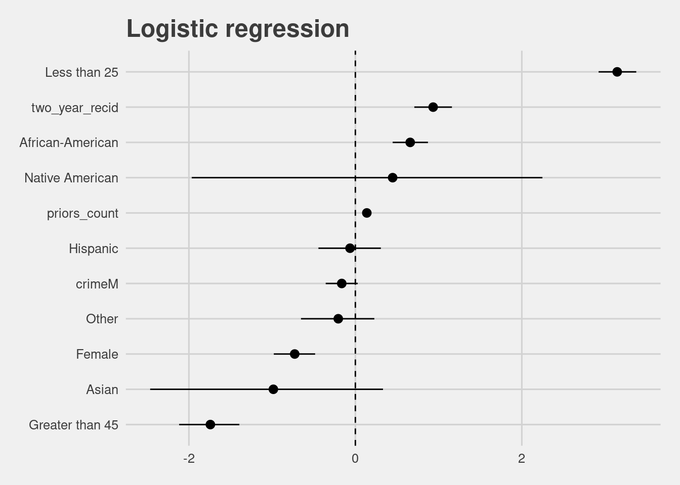
interpret_estimate <- function(model){
# Control
intercept <- model$estimate[model$term == "(Intercept)"]
control <- exp(intercept) / (1 + exp(intercept))
# Likelihood
model <- model %>% filter(term != "(Intercept)")
model$likelihood <- (exp(model$estimate) / (1 - control + (control * exp(model$estimate))))
return(model)
}
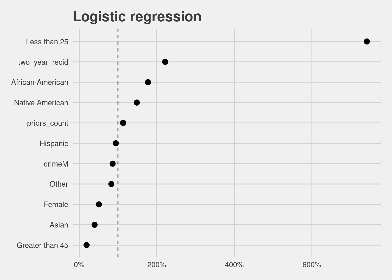
interpret_estimate(lr_model) %>%
mutate(term = gsub("race|age_cat|gender","", term)) %>%
ggplot(aes(x = fct_reorder(term, likelihood), y = likelihood)) +
geom_point(size = 3) +
coord_flip() +
labs(y = "Likelihood", x = "",
title ="Logistic regression") +
scale_y_continuous(labels = scales::percent_format(accuracy = 1)) +
geom_hline(yintercept = 1, linetype = "dashed")